Keywords: tests, hypothesis, level, significance, region.

Abstract

In class sessions on Statistics and Probability in the content of Hypothesis Testing, the following question is asked to the professor, why use such a small significance level in most of the proposed exercises? The teacher answers: “to be almost 100% sure”, an answer almost similar to the one given in the bibliographies related to the subject, but in this study, a criticism or observation is made to the effect that this answer is inadequate and, on the contrary, the significance level should not be so small. The objective of this document is to reflect on how we teach in Statistics and Probability the content of Hypothesis Testing or to support this gap of knowledge that is present and is not addressed in any book, based on the exhaustive consultations made in the Mathematics and Statistics with Probabilities bibliographies in the virtual libraries of the library system of the universities registered to the CNU (National Council of Universities), Central Library of the UNAN-Managua and virtual libraries of other international universities. The bibliography related to this critical content is very scarce since the revision proposal is an original idea of the author in this study article. This can also be argued by the Ph.D. in Mathematics and Statistics Elisa Cabana in the article Why a significance level of 0.05? (Cabana, 2021), where she expresses that there is no scientific basis for the choices made by Fisher (English Mathematician) in his texts on the Normal distribution. Within the process of hypothesis testing, the types of hypotheses and the different methods to be used to determine whether a hypothesis is rejected or there is not enough argument to accept it are considered. In all these processes the significance level (many times represented by the Greek letter Alpha (α)) is considered as a value between 1%, 5%, or 10% (Harcet et al., 2014, p. 101). The significance value is the representation in the area of the rejection region on a Gaussian curve. Hypothesis testing is related to confidence intervals that support the decision to reject the null hypothesis if the presumed value for the population mean is outside the confidence interval with a significance level of α%. This paper will provide some solved examples to support the analysis of the situation at hand.

So a very small significance level only opens a very wide range to make inference or estimation about the population mean from the sample mean of a random variable.

Therefore, the consideration addressed and raised in this paper is the use of an α>10% to surrounding more precisely the population mean and thus be able to infer or estimate with greater precision and certainty the value of the population mean.

Introduction

Hypothesis Testing

The establishment and testing of hypotheses is an essential part of statistical studies. To formulate such a test, a theory is usually proposed, which has not yet been proven to be true. For example, suppose it has been claimed that a new drug to help fight infection works better than the current drug. We want to establish and test a hypothesis to determine whether this claim is true.

Hypothesis testing always begins with a statement about a population parameter. In general, when hypotheses are discussed, two statements that are directly contradictory to each other are considered. The process of hypothesis testing provides us with arguments as to why a certain hypothesis can be accepted or rejected.

The hypothesis stated is called the null hypothesis and we denote it by H0 and the alternative hypothesis states the opposite and is denoted by H1.

Let us consider an example of broiler chickens. Suppose that data from previous years indicate that the average weight of the broiler population is 2 kg. We want to estimate the average weight of this year’s broilers, and for this, we take a sample of a certain size. The sample mean is 2.0 kg. The null hypothesis always states that there is no change, i.e., the mean weight of broilers this year is also 2 kg. We write it as H0:μ=  (where μ is the population mean and  is the sample mean).

The alternative hypothesis can have different statements depending on the type of test we want to perform.

There are two types of hypothesis tests and three types of alternative hypotheses

i. Two-tailed test (H1:μ≠ ): in the example it means that the mean weight of chickens is different from 2 kg.

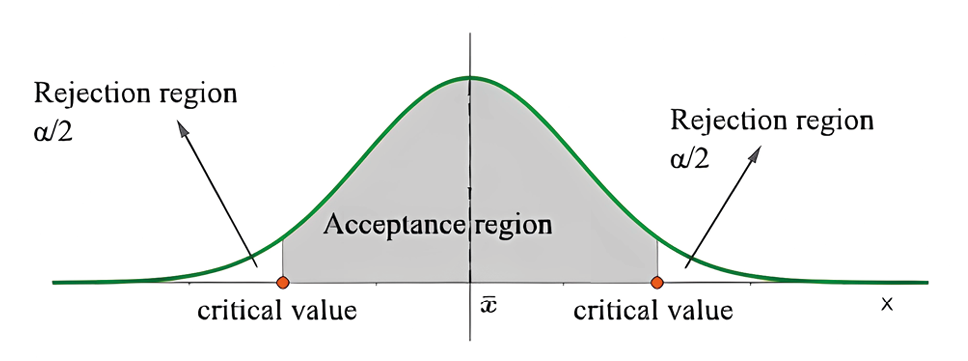
Figure 1. Two-tailed hypothesis test.

ii. One-tailed upper test (H1:μ>x̅ ): the mean weight of chickens is greater than 2kg.

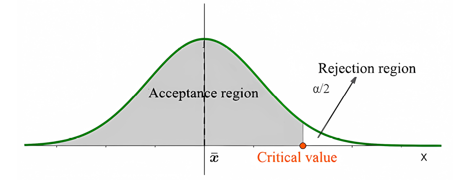
Figure 2. One-tailed upper-tailed hypothesis testing.

iii. Testing of a lower tail (H1:μ<x̅ ): mean chick weight is less than 2kg.

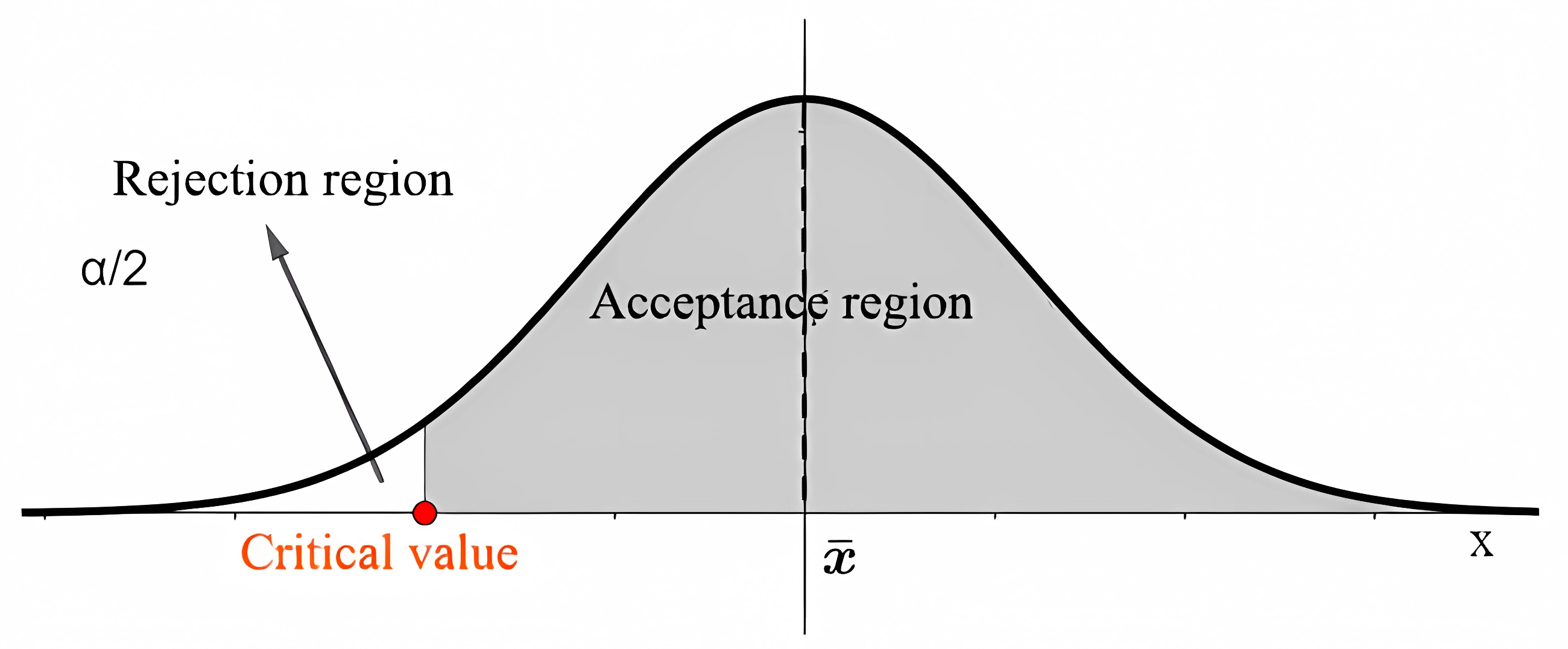
Figure 3. One-tailed lower-tailed hypothesis test.

We must also decide what significance level, α, we need to conclude that a given hypothesis is accepted, with ( 1 - α) % certainty. The significance level is directly related to the confidence interval, so if we are 95% sure that the mean value is in the confidence interval we can accept the null hypothesis with a significance level of 5% of the test.

The significance levels are usually 1%, 5%, and 10%. When calculating test statistics, as well as calculating confidence intervals, we use the z-statistic if not the t-statistic. We will use the z-statistic when the variance is known, and the t-statistic when the variance is unknown (regardless of sample size, the latter is not relevant in this study).

There are two ways to make a decision based on the calculated values.

I.The critical value is the z-value or t-value found at the significance level of the test. If the z-value or t-value of the test is outside the so-called acceptance region, we reject the null hypothesis, otherwise, we do not reject it.

II.The p-value is the probability that the parameter we are investigating (i.e. the mean) lies within the rejection region, given that the null hypothesis is true. If the p-value is greater than the significance level we cannot say that we accept the null hypothesis, but rather we say that “we do not have sufficient evidence to reject”, or simply “we do not reject”, the null hypothesis.

We have four steps to follow in a hypothesis test

Step 1. Establish the null and alternative hypothesis

Step 2. Establish a criterion for a decision

Step 3. Calculate the necessary statistics

Step 4. Decide or make a decision based on the calculated statistics and decision criteria.

Significance level: The significance level is the cutoff for judging a result as statistically significant. If the significance value is less than the significance level, the result is considered to be statistically significant. The significance level is also known as the alpha level (Cognos Analytics, 2021).

Hypothesis testing for when the mean and variance are known.

As in the calculation of confidence intervals, we use z-statistic in hypothesis testing. Let’s look at an example in which we will relate it to the confidence interval.

Next, we will present a couple of examples in the development part, with the methods indicated in the bibliographies, in which we deal with the analysis and conclusion of the same.

Development

Example 1a

It is known that the drying time of a type of car paint has a normal distribution with a mean of 75 minutes and a standard deviation of 9 minutes. Car painters at an automotive company have discovered an additive that shortens the drying time. However, if the company approves the use of this additive, the cost of painting a car will naturally increase. They will not approve it unless they have solid evidence that the additive reduces drying time. A test on 49 new cars gave an average drying time of 72 minutes.

Using a 5% significance level, what would you recommend to the company?

Solution

We establish the null and affirmative hypotheses

H0: μ=75

H1: μ<75

Using the Texas Instrument calculator, we obtain the following results,

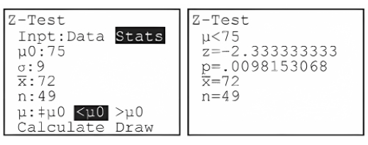
Performing the probabilistic p-value comparisons at the significance level α

0.0098<0.05

Since this value is less than 5%, we reject the null hypothesis and conclude that we have sufficient evidence that the average drying time is less than 75 minutes. Therefore, the company can go ahead and start using the additive.

Example 2b

In a certain country, the mean height of the population of men is believed to be 182 cm, and the standard deviation is 5 cm. A random sample of 100 men was drawn from the population and the mean height was found to be 183.6 cm.

a.State the null and alternative hypothesis

b.Use a two-tailed test with a 10% significance level to decide whether the statement is true or not.

Solution a

Our null hypothesis H0 is to maintain the statement that the population mean (μ) is 182 cm expressed as follows.

H0: μ=182

The alternative hypothesis states the opposite of the null hypothesis, in this case as a two-tailed test is requested it is stated as:

H1: μ≠182

Graphically with a significance level of 10%, this means the following.

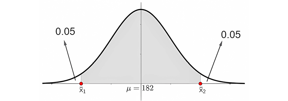
Figure 4. Representation of the provided problem information.

Performing a standardization for z where z1 ≡ x1 and z2 ≡ x2 we have the following:

The sample standard deviation is calculated as follows.

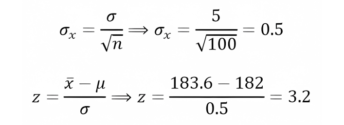
Since α=0.1, it is the region of rejection spread over the two tails,

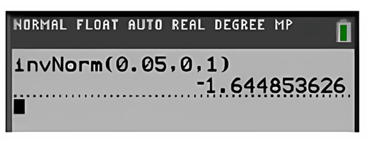
The standardized value of z1~zα/2 for an area of 0.05 is

Because of its symmetry z1=1.645, we proceed to compare z and z1, resulting respectively in the comparison 3.2>1.645, graphically we can see it like this

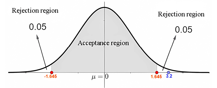
Figure 5. Information on a standardized normal curve

The value of z=3.2 which is the standardization of 197.5 is outside the acceptance region so the null hypothesis is rejected at a significance level of 10%.

This conclusion can be extended to the confidence intervals. In the previous example, when returning the standardization to the random variable X, it is observed as follows

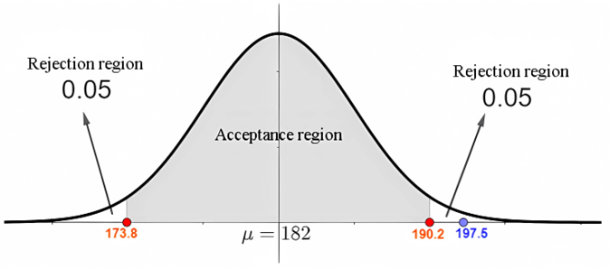
Figure 6. Result information for the unstandardized curve

Performing the calculation of confidence intervals in this situation by applying the use of the statistical calculator we obtain the following information.

Figure 7. Results provided by the Texas instruments calculator

The confidence interval confirms once again that the established null hypothesis must be rejected since what is believed to be the population mean (μ=182) is outside the confidence interval (182.78,184.42).

It is known that in a confidence interval the larger the sample size the more precise inference will be made about the population mean of a random variable under study, for example, a survey is conducted in a certain country, the more people we integrate into the survey the more precise will be the value of the sample mean of a random variable under study towards the mean of the entire population of that random variable.

We proceed to review the following example number three.

EXAMPLE 3c

When we compare the p-value at each of the common significance levels (1%, 5%, and 10%), we conclude that we reject the null hypothesis at all three significance levels, since 0.0037 is less than every one of them.

After a night of rain, 12 earthworms surfaced in the soil. Their lengths, measured in cm, were as follows: 12.0, 11.1, 10.5, 10.8, 12.1, 10.4, 10.9, 12.2, 10.9, 11.9, 11.12, and 11.6. The worms are known to be from a population that follows a normal distribution with the mean value of 10.5 cm and a standard deviation of 2cm. The worms are believed to be increasing in size.

a.State the null and alternative hypotheses.

b.Use a one-tailed upper test at the 5% significance level to decide whether the statement is true or not.

Solution

H0: μ=10.5

H1: μ>10.5, is the belief that the worms are increasing in size.

Solution b

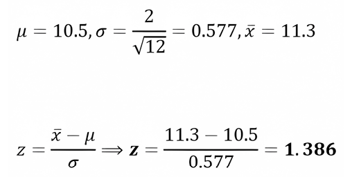
The critical z value given that it is one-tailed has as value α=0.05→zα=z0.95=1.645.

Comparing zα > z, 1.645>1.386 with this we conclude that we do not have enough evidence to reject the null hypothesis at 5% significance level.

Checking the problem by the method of p, we obtain using the statistical calculator, Texas instrument

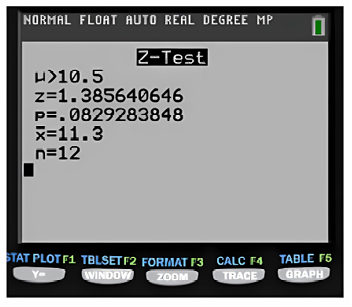
Figure 8. Comparison of results with the Texas instruments calculator.

Performing the comparison of p and α results 0.0829>0.05, we can conclude in the problem that we do not have enough evidence to reject the hypothesis.

The example ends here.

But let’s analyze the issue a little further!!!!

Now let’s add to this previous example a third subsection with the following statement.

c.Now use a significance level of 10% and perform the comparisons and conclusion criteria again.

To provide a solution, by performing the comparisons it turns out to have: 0.0829<0.10, in this case, it changes the conclusion to reject the null hypothesis, and so it remains for all cases where the significance level is greater than 10%.

Conclusions

Maintaining an Alpha significance level between the range of 1%-9% is completely suboptimal for the inference of a parameter such as the sample mean to the population mean. In Example 2 of the development we can see that if we change the significance level to an α=10%, the conclusion in the problem changes to outright rejecting the null hypothesis and this decision would hold for any significance level greater than 10%. We can interpret this as if we have a wide range of options for inferring on the population mean and whichever one is proposed would be accepted, while a not-so-small significance level defined as greater than 10% reduces those multiple options to a smaller range where we can infer more accurately or closer to the population mean. We can also see it with this example: if I tell you that I think of a number from 1 to 1000 and you tell me what that number is, your answer might not be assertive enough to infer the number I think of, whereas, if I tell you that I think of a number from 1 to 5 your answer would be closer to or exactly match the number I have in mind.

Based on Dr. Cabana’s article, where she expresses: “that these significance values can neither be arbitrary nor agreed upon. Although in the scientific community, the standard value is generally used in many fields, possibly because it is a subject still debated today...” (Cabana, 2021) That is why we cannot maintain the theory that the significance level should be between 1% and 10%, on the contrary, if we want to infer faithfully to the population mean we must choose a significance level greater than or equal to 10% and not stay with these very low significance level values.

Having a very small significance level rather generates a lot of confidence, which in this type of situation would not be correct to be too confident, since we would accept any proposal that is offered because we are too confident.

The debate, proposals, and analysis are open to the people who review this document.

---